CSV Openturns Kriging

Dear all,

I have a csv file with three columns.
the first two being x and y coordinates, the third column is my observation at specific location.

here is a sample csv of my data:
samplecsv.csv (2.8 KB)

I want to perform perform a spherical Kriging Interpolation using openturns, showing me the spatial Interpolation of the data.
However, I’m not sure how to load my data into my script as an ot.Sample. I assume that my points are spatially correlated, normalized and have no trend.

Hi @ericmoon!

Here is a step-by-step guide.

Load the sample

import openturns as ot
sample = ot.Sample.ImportFromTextFile('samplecsv.csv', ',', 2)

Your CSV file is a little nonstandard: there are 5 rows and 58 columns separated by commas,
so the second argument must be the separator ‘,’

From your post, I gather that only the last 3 lines are needed, so the third argument is to skip the first 2 lines.

Now, OT expects the Sample columns to represent dimensions, so we need to transpose the table. There is no native way to do it in OT, but this can fortunately be delegated to numpy.

import numpy as np
arr = np.array(sample).T # convert Sample into np array and transpose

Split the data into input and output Samples

input_sample = ot.Sample(arr[:, 0:2])
output_sample = ot.Sample(arr[:, 2:])

Two things can be noted here:

  1. It is not strictly necessary to turn the numpy arrays back into OpenTURNS Samples, since OT knows to interpret 2D numpy arrays as Samples (and 1D numpy arrays as Points), but doing it is a way to make sure we have valid Samples.
  2. Even though the output is represented by a single column, we need to extract it as a 2D numpy array, otherwise it will be understood as a single 58-dimensional Point. Hence the “2:” instead of “2”. Try removing the column: you will see the command fails without it.

Simple Kriging: create the null Basis

basis = ot.Basis(0)

Specify the covariance kernel (“model” in the API)

cov = ot.SphericalModel(2) # parameters to be estimated later: specify only dimension

Create and run the Kriging model

kri = ot.KrigingAlgorithm(input_sample, output_sample, cov, basis)
kri.run()

Get the result (contains all the information) and specifically, the metamodel

res = kri.getResult()
metamodel = res.getMetaModel()

Plot the metamodel

lower = [-10.0] * 2 # lower bound of the 2D window
upper = [10.0] * 2 # upper bound of the 2D window
graph = metamodel.draw(lower, upper)
graph.setBoundingBox(ot.Interval(lower, upper))
graph.add(ot.Cloud(input_sample)) # overlay a scatter plot of the observation points
graph.setTitle("Kriging metamodel")

# A View object allows us to interact with the underlying matplotlib figure 
from openturns.viewer import View
view = View(graph, legend_kw={'bbox_to_anchor':(1,1), 'loc':"upper left"})
view.getFigure().tight_layout()

image

1 Like

Dear @josephmure

First, I must thank you kindly for the step-by-step guide! It helped alot along reading up on the documentation. Especially the part with seperating the csv did clarify a lot!

Yet I do have some follow-up questions:

  1. the actual file contains more than 140.000 points(rows)
    I don’t get any results - is there a limit in reading range?

  2. If I want to use a universal kriging with a quadratic drift, how(with what) do I change the covariance kernel varible?

  3. the plotted metamodel looks good, but what if I want to present it with a really smooth surface and a gradient effect such in here:

  4. is there a way to transform this into a “map” with longitude and latitude values on the x and y axis?

again, Thanks for the help!

Hi @ericmoon!

  1. I am aware of no such limit. Do you get an error message? If so, can you please post it? If Sample.ImportFromTextFile remains unsuccessful, you can try using numpy or pandas.read_csv. As mentioned in my previous post, 2D numpy arrays are interpreted by OT as Samples anyway, and you can convert a pandas DataFrame to a numpy array with pandas.DataFrame.to_numpy() EDIT: For really large datasets, you may want to perform Kriging with HMAT, but I will let specialists @KieranDelamotte @regislebrun @sofianehaddad give more details.

  2. Have a look at the Kriging quick start example:
    basis = ot.QuadraticBasisFactory(dimension).build()

  3. OpenTURNS has a few graphical utilities (actually convenient wrappers to matplotlib), but heatmaps are not among them. You will need to directly use matplotlib or some other graphical library. Here is a script that works with matplotlib on your example (it draws inspiration on the example Kriging with an isotropic covariance function — OpenTURNS 1.17 documentation):

import matplotlib.cm as cm
import matplotlib.pyplot as plt

# Matplotlib expects X and Y coordinates to be arranged as a numpy meshgrid.
delta = (upper[0] - lower[0]) / 100
x = y = np.arange(lower[0], upper[0], delta)
X, Y = np.meshgrid(x, y)

# OT however requires Points/Samples or 1D/2D numpy arrays.
# The following lines convert the meshgrid (X, Y) to a 2D numpy array xy.
x = X.reshape(-1)
y = Y.reshape(-1)
xy = np.zeros((len(x), 2))
xy[:, 0] = x 
xy[:, 1] = y

# Apply the metamodel to all points in xy
# and turn the resulting Sample into a numpy array z.
z = np.array(metamodel(xy))

# Reshape z to make Matplotlib understand it represents a field.
Z = z.reshape(X.shape)

# Plot the heatmap.
fig, ax = plt.subplots()
im = ax.imshow(Z, interpolation='bilinear', cmap=cm.seismic,
               origin='lower', extent=[lower[0], upper[0], lower[1], upper[1]],
               vmax=abs(Z).max(), vmin=-abs(Z).max())

spherical_heatmap

  1. I am not sure I understand this question. Is it related to your question about heatmaps?
1 Like

Dear @josephmure ,

once again, thnaks for the help!

  1. Not so sure how to deal with this:

I will have a look at HMAT, I’ve not heard of it, yet.

  1. Kinda it is realted to heatmaps, correct. So what I want to end up finally is a raster file or some similiar format where I can overlay the heatmap on a Openstreetmap in QGIS. Hence why I’m interested in the longitude and latitude values of the graph.
    A good example is here:

Thank you for the help!

Hi @ericmoon,

The output you posted shows two lines related to upper bouds. The first one mention an upper bound of dimension 3, the second one of dimension at least several hundreds. It is a sign that you forgot to transpose your data somewhere.
The sample file you joined to your first message contains (from an OpenTURNS perspective) one line of description followed by four rows of data, the first of them being ignored as it contains a NaN. As this line contains essentially integers, I assume that they are some sort of indices that should be ignored. Joseph already shown you how to select specific components and how to transpose your data, so please double check that you followed his recommendations.
Concerning the kriging of large data sets, there are several aspects to take into account:

  • in 2 dimensions, such a large number of evaluations should allow you to use much cheaper approximations and still get meaningful results. For example, you could triangulate your locations using scipy.spatial.Delaunay then use the P1LagrangeEvaluation class in OpenTURNS to get a piecewise linear interpolation of your data. Thanks to its very efficient kd-tree, the evaluation of this function is O(log(n)) where n is your number of points (n=130000)
  • if you manage to get a kriging interpolation, its evaluation cost may be prohibitive for your needs as it scales as O(n)
    If you really want to use kriging, then you must use the HMAT linear algebra backend (i.e. compressed algebra) as the use of dense algebra (the default) will need 260Go of RAM to store the covariance matrix and its Cholesky factor. To use this backend, have a look at Kriging the cantilever beam model using HMAT — OpenTURNS 1.17 documentation, in particular the following lines:
ot.ResourceMap.SetAsString("KrigingAlgorithm-LinearAlgebra",  "HMAT")
ot.ResourceMap.SetAsScalar("HMatrix-AssemblyEpsilon",  1e-3)
ot.ResourceMap.SetAsScalar( "HMatrix-RecompressionEpsilon",  1e-4)

You should use a much smaller value for HMatrix-AssemblyEpsilon and HMatrix-RecompressionEpsilon, let’s say 1e-6 and 1e-7, in order to be sure that the compression of the matrix did not introduced too much error. This way, you replace the O(n^2) storage by an O(nlog(n)) storage and the O(n^3) factorization time (with a small constant thanks to parallelism in the BLAS) by an O(nlog^2(n)) but with a quite large constant as the implementation of HMAT shipped with OpenTURNS is sequential.

Be aware of the fact that it is quite tricky to see if the compression worked well. The use of small epsilons is a first guard, but you have to double check the results, for example by using the largest subset of your data you can use with dense algebra and by comparing the results you get with the ones of HMAT on this subset and for this choice of epsilons.

If you are able to share your data I can do a part of the job for you :wink:

IMO, your last question is loosely related to OpenTURNS as once you know how to evaluate your metamodel, the conversion into any kind of external format is a pure python task. If you post the source code you used to get your last pretty picture I can try something on my side.

Cheers

Régis

1 Like

Dear @regislebrun

thank you very much for all your information.
I have to look into the HMAT intesively.
I also get a look into the Delauney triangulation and Lagrange evaluation for interpolating.
Yet I do really want to look into Kriging, I performed it at selected key areas and now I want to perform kriging interpolation with all points I’ve gathered.

"260Go of RAM " -what exactly does that mean?

I’d be most grateful for a little help around and a head start, here is my data:

I cleaned the data, but it’s still too big so here is a download link, hope its ok (:

Again, these are longitude, latitude and deformation rates.

Sadly its just a picture I found online in an article with no well citation.

Best regards and thank you kindly!

Eric

Hi Eric,
The 260Go (in fact, 270Go) of RAM are the quantity of memory you need to store the covariance matrix and its Cholesky factor in dense format for the kriging of a database containing 130000 points: 130000x130000x8=135Go (as a double precision floating point is 8 octets long) for each matrix, for a total of 2x135=270Go. In fact the database contains 141683 points so the memory requirement is 321Go, much more than what is available on standard workstations.
I am currently playing with your data and kriging+the HMAT compression. As expected, it perfectly fits into my 128Go of RAM (in fact it needs only 16Go in compressed form using the small epsilons I suggested) but the resolution still takes some time. As I am currently on vacations and for the next two weeks, hiking in the Alps, don’t expect too much activity from my side. I have only some half hour slots in the evening to try things, and my laptop has the night to crunch it ;-)!

Cheers

Régis

1 Like

Dear @regislebrun

thank you again, for the context. I did not expect to be it this hungry in memory!

I’m no trying out the Delaunay and Lagrange evaluation as you said, but I’m having trouble in understanding it correctly by myself.

I triangulate my area and perform a lagrange evaluation, how exactly is it then connected to the kriging interpolation? And what exactly is the lagrange method evaluating?

I tried it piece by piece for my self. but I get an error message regarding Qhull.

import openturns as ot 

sample = ot.Sample.ImportFromTextFile('cleandata.csv', ',', 2)
arr = np.array(sample).T

#print(arr)

from scipy.spatial import Delaunay  

tri = Delaunay(arr)

evaluation = ot.P1LagrangeEvaluation(tri)

print(evaluation)

Edit: Here is the error Message:

I’d be thankful, if you would be willing to clarify these misunderstandings of mine.

p.s.: Great to hear you have fun with my data :slight_smile: and have a great trip! I did hike in the alps a couple of years ago too.

Dear all,

after a short summer break on my end, I’m back on my project.
in the meantime, I was able to gather new points in elevation for the study area and read on a lot about kriging.

Now, I have several study areas I want to look at with ordinary kriging(spherical semivariogram model).

It’s “only” 700-100 points each so I tried it with zour post , @josephmure and still got an error.
Unfortunately, I still need a bit of clarification what these errors mean and how to get this 100% in advance for all of my other study areas.

here is the csv-file a4buir.csv (43.5 KB)

and here is my code so far:

"""Coding the spatial interpolation : Krigging of study areas"""

import openturns as ot


import numpy as np

arr  = np.loadtxt('a4buir.csv', delimiter= ",", skiprows=1)
input_sample = ot.Sample(arr[:, 0:2])
output_sample = ot.Sample(arr[:, 2:])

basis = ot.Basis(0)

cov = ot.SphericalModel(2) 


#Check the list of parameters to be estimated:

#print(cov.getParameterDescription())
#print(cov.getFullParameterDescription())

cov.setActiveParameter([0, 1, 2, 3])
#print(cov.getParameterDescription())

kri = ot.KrigingAlgorithm(input_sample, output_sample, cov, basis)
kri.run()

res = kri.getResult()
metamodel = res.getMetaModel()

lower = [-20.0] * 2 
upper = [50.0] * 2 
graph = metamodel.draw(lower, upper)
graph.setBoundingBox(ot.Interval(lower, upper))
graph.add(ot.Cloud(input_sample)) 
graph.setTitle("Kriging metamodel")


from openturns.viewer import View
view = View(graph, legend_kw={'bbox_to_anchor':(1,1), 'loc':"upper left"})
view.getFigure().tight_layout()

import matplotlib.cm as cm
import matplotlib.pyplot as plt

delta = (upper[0] - lower[0]) / 100
x = y = np.arange(lower[0], upper[0], delta)
X, Y = np.meshgrid(x, y)


x = X.reshape(-1)
y = Y.reshape(-1)
xy = np.zeros((len(x), 2))
xy[:, 0] = x 
xy[:, 1] = y


z = np.array(metamodel(xy))


Z = z.reshape(X.shape)


fig, ax = plt.subplots()
im = ax.imshow(Z, interpolation='bilinear', cmap=cm.seismic,
               origin='lower', extent=[lower[0], upper[0], lower[1], upper[1]],
               vmax=abs(Z).max(), vmin=-abs(Z).max())

and here is the error I get:

thanks again for all the help and take take

best regards Eric

edit I tried diffrent limits but I can’t seem to get good results:

Kriging model looks like this:

and the heatmap like this:

Hi Eric,

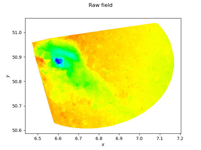
I am back from my trip. Here is what your data look like using a Delaunay triangulation to rebuild the underlying mesh:
field

Using a P1 interpolation:

import openturns as ot
import openturns.viewer as otv
import numpy as np
from scipy.spatial import Delaunay

sample = ot.Sample.ImportFromTextFile('cleandata.csv', ',', 2)
points = sample.getMarginal([1, 2])

visuMesh = False

print("Build triangulation")
tri = Delaunay(points)
print("Build mesh")
mesh = ot.Mesh(points, [[int(x) for x in t] for t in tri.simplices])
if visuMesh:
    import matplotlib.pyplot as plt
    plt.triplot(points[:,0].asPoint(), points[:,1].asPoint(), tri.simplices)
    plt.plot(points[:,0], points[:,1], 'o')
    plt.show()
    ot.ResourceMap.SetAsUnsignedInteger("Mesh-LargeSize", 0)
    ot.Show(mesh.draw())
field = ot.Field(mesh, sample.getMarginal(3))
print("Display raw field")
g = field.draw()
g.setXTitle(r"$x$")
g.setYTitle(r"$y$")
g.setTitle("Raw field")
view = otv.View(g)
view.save("field.png")
view.close()
print("Min/Max values")
print(field.getValues().getMin(), field.getValues().getMax())
print("Build P1 interpolation")
function = ot.Function(ot.P1LagrangeEvaluation(field))
xyMin = points.getMin()
xyMax = points.getMax()
M = 256
square = ot.IntervalMesher([M]*2).build(ot.Interval(xyMin, xyMax))
fieldP1 = ot.Field(square, function(square.getVertices()))
g = fieldP1.draw()
g.setXTitle(r"$x$")
g.setYTitle(r"$y$")
g.setTitle("Interpolated field")
view = otv.View(g)
view.save("fieldP1.png")
view.close()

you get:
fieldP1
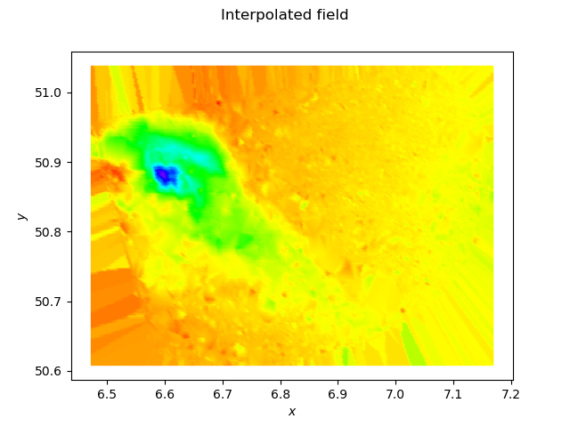
You see the blurry effect due to the linear interpolation, and the rays outside of the mesh due to the extension of the piecewise linear function by a piecewise constant function in these regions.

I also tried to use KrigingAlgorithm with HMAT on your data. Unfortunately there is a bug with SphericalModel and I get an exception. Switching to a MaternModel with nu=3/2 to get approximately the same level of smoothness I get the following computation time, depending of the size of the subsample I use:

# Matern 3/2 oss
#   1000 0.9618020057678223
#  10000 20.189648628234863
#  20000 48.61438536643982
#  50000 399.1733877658844
# 100000 1231.114249944687
#   full 1172.22917294502264

so you see that it works (i.e. it fits into the memory and it returns an answer in a finite amount of time) but it is expensive, and the resulting meta-model is slow. The output is:
fieldKriging
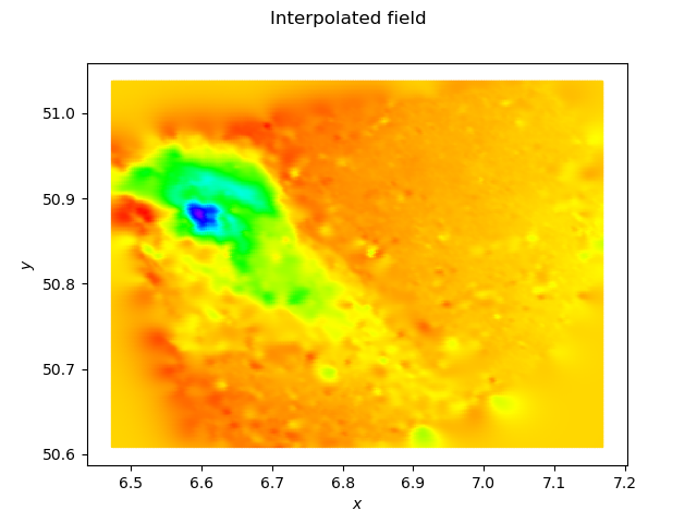
which is quite similar to the P1 result on the initial mesh, and a little bit smoother outside of the mesh. The script I used is:

import openturns as ot
import openturns.viewer as otv
import numpy as np
import time

# Here we use numpy to transpose data
sample = ot.Sample.ImportFromTextFile('cleandata.csv', ',', 2)
points = sample.getMarginal([1, 2])

dim = points.getDimension()
z = sample.getMarginal(3)
delta = points.computeRange()
xyMin = points.getMin()
xyMax = points.getMax()
print("points=", points.getSize())
print("z=", z.getSize())
print("delta=", delta)
# Spherical kernel
#kernel = ot.SphericalModel(2)
#kernel.setActiveParameter([0,1,2,3])
#kernel.setParameter([0.1]*4)
kernel = ot.MaternModel([0.1]*2, [1.0], 1.5)
#kernel.setActiveParameter([])
#kernel.setParameter([0.1, 0.1, 1.0, 1.5])
ot.ResourceMap.SetAsString("KrigingAlgorithm-LinearAlgebra",  "HMAT")
ot.ResourceMap.SetAsScalar("HMatrix-AssemblyEpsilon",  1e-6)
ot.ResourceMap.SetAsScalar( "HMatrix-RecompressionEpsilon",  1e-7)
algo = ot.KrigingAlgorithm(points, z, kernel, ot.Basis())
optimizer = ot.NLopt("LN_COBYLA")
algo.setOptimizationAlgorithm(optimizer)
ot.Log.Show(ot.Log.INFO)
t0 = time.time()
algo.run()
t1 = time.time()
print("t=", t1 - t0, "s")
metaModel = algo.getResult().getMetaModel()
M = 256
square = ot.IntervalMesher([M]*2).build(ot.Interval(xyMin, xyMax))
fieldP1 = ot.Field(square, metaModel(square.getVertices()))
g = fieldP1.draw()
g.setXTitle(r"$x$")
g.setYTitle(r"$y$")
g.setTitle("Interpolated field")
view = otv.View(g)
view.save("fieldKriging.png")
view.close()

Cheers

Régis

1 Like

Dear Régis,

Merci bien.
I thank you kindly, it helps me alot!
As expected I don’t seem to have enough memory for the coomplete dataset, but since I decided to break it in specific pieces(areas), it’s no longer an issue anyway.
Out of curiousity:
what do the following lines in the kriging code do?

optimizer = ot.NLopt("LN_COBYLA")
...
square = ot.IntervalMesher([M]*2).build(ot.Interval(xyMin, xyMax))

One last question:
since I will georeference it, I want to inverse the colors(very low values = red, high elevation values = blue).
How do I inverse the colors?

Best regards

Simon

Hi Eric,

To answer your first question, recent experiments conducted at ONERA showed that the NLopt implementation of the Cobyla optimization algorithm works best for Kriging hyperparameter optimization. OpenTURNS also has a native implementation of Cobyla (accessible as ot.Cobyla()) but the NLopt version performs better. Work has been started in order to bring the improvements of the NLopt version to the OT native version, so stay tuned for that. Currently, however, it is best to manually specify that you want your KrigingAlgorithm to use the NLopt version of Cobyla.

The IntervalMesher class allows to create a mesh for a given box. Here, square is the resulting mesh, which is then used to support a field. Have a look at the following example to see how the class van be used:

https://openturns.github.io/openturns/1.17/auto_probabilistic_modeling/stochastic_processes/plot_create_mesh.html

As for your second question, I do not know but you can always recover the matplotlib figure from the OpenTURNS View object thanks to the getFigure() method. Then I suppose you can modify the matplotlib colormap, but I do not know the exact code lines you need.